Oorspronklike lêer(2 406 × 1 978 piksels, lêergrootte: 55 KG, MIME-tipe: image/png)

Hierdie lêer kom vanaf Wikimedia Commons en kan ook in ander projekte gebruik word. Die beskrywing op die lêer se inligtingsblad word hieronder weergegee.

Opsomming

File:Newton iteration.svg is a vector version of this file. It should be used in place of this PNG file when not inferior.

File:Newton iteration.png → File:Newton iteration.svg

For more information, see Help:SVG.
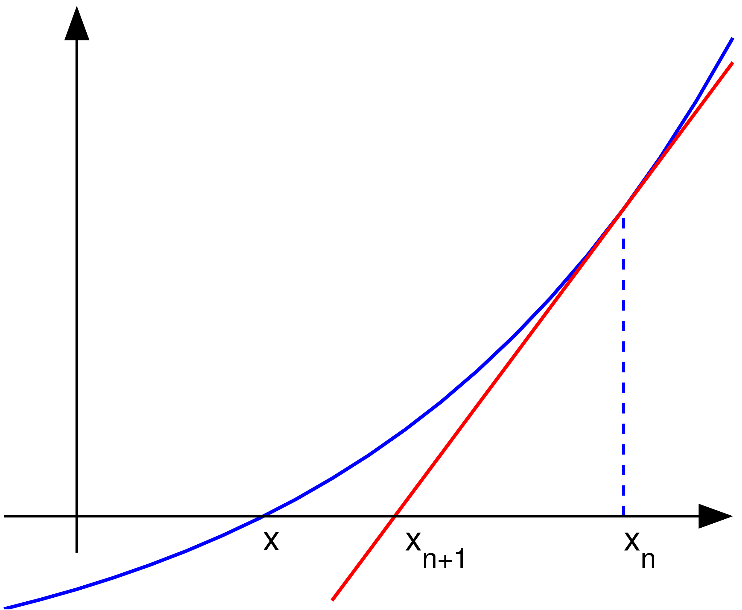
In other languages
Alemannisch  Bahasa Indonesia  Bahasa Melayu  British English  català  čeština  dansk  Deutsch  eesti  English  español  Esperanto  euskara  français  Frysk  galego  hrvatski  Ido  italiano  lietuvių  magyar  Nederlands  norsk bokmål  norsk nynorsk  occitan  Plattdüütsch  polski  português  português do Brasil  română  Scots  sicilianu  slovenčina  slovenščina  suomi  svenska  Tiếng Việt  Türkçe  vèneto  Ελληνικά  беларуская (тарашкевіца)  български  македонски  нохчийн  русский  српски / srpski  татарча/tatarça  українська  ქართული  հայերեն  বাংলা  தமிழ்  മലയാളം  ไทย  한국어  日本語  简体中文  繁體中文  עברית  العربية  فارسی  +/−
New SVG image

Beskrywing Uploader graphed this with en:MATLAB (Illustration of en:Newton's method)
Datum 22 November 2004 (first version); 2004-11-23 (last version)
Bron Transferred from en.wikipedia to Commons.
Outeur Olegalexandrov at Engels Wikipedia
PNG genesis
InfoField
 
This diagram was created with MATLAB.
Bronkode
InfoField

MATLAB code

(Newton iteration)
% illustration of Newton's method for finding a zero of a function

function main ()
   
a=-1; b=1;   % interval endpoints
fs=20;       % text font size

% arrows settings
thickness1=2; thickness2=1.5; arrowsize=0.1; arrow_type=1;
angle=20; % in degrees

h=0.1;  % grid size
X=a:h:b; % points on the x axis
f=inline('exp(x)/1.5-0.5');   % function to plot
g=inline('exp(x)/1.5');       % derivative of f
x0=0.7; y0=f(x0);             % point at which to draw the tangent line 
m=g(x0);
Y=f(X);                       % points on the function to plot
XT=-0.1:h:b; YT=y0+(XT-x0)*m; % tangent line

% prepare the screen
clf; hold on; axis equal; axis off

% plot the graph and the tangent lines
plot(X, Y, 'linewidth', thickness1)
plot(XT, YT, 'r', 'linewidth', thickness1)
plot([x0 x0], [0, y0], '--', 'linewidth', thickness2)

% axes
small=0.2;
arrow([a 0], [b, 0], thickness2, arrowsize, angle, arrow_type, [0, 0, 0])
arrow([a+small, -0.1], [a+small, 1.4], thickness2, arrowsize, angle, arrow_type, [0, 0, 0])

% text
H=text(-0.29, -0.06,  'x'); set(H, 'fontsize', fs)
H=text(0.1, -0.1,  'x_{n+1}'); set(H, 'fontsize', fs)
H=text(0.7, -0.1,  'x_{n}'); set(H, 'fontsize', fs)

% save to disk
saveas(gcf, 'newton_iteration.eps', 'psc2')

function arrow(start, stop, thickness, arrow_size, sharpness, arrow_type, color)

% Function arguments:
% start, stop:  start and end coordinates of arrow, vectors of size 2
% thickness:    thickness of arrow stick
% arrow_size:   the size of the two sides of the angle in this picture ->
% sharpness:    angle between the arrow stick and arrow side, in degrees
% arrow_type:   1 for filled arrow, otherwise the arrow will be just two segments
% color:        arrow color, a vector of length three with values in [0, 1]

% convert to complex numbers
   i=sqrt(-1);
   start=start(1)+i*start(2); stop=stop(1)+i*stop(2);
   rotate_angle=exp(i*pi*sharpness/180);

% points making up the arrow tip (besides the "stop" point)
   point1 = stop - (arrow_size*rotate_angle)*(stop-start)/abs(stop-start);
   point2 = stop - (arrow_size/rotate_angle)*(stop-start)/abs(stop-start);

   if arrow_type==1 % filled arrow

      % plot the stick, but not till the end, looks bad
      t=0.5*arrow_size*cos(pi*sharpness/180)/abs(stop-start); stop1=t*start+(1-t)*stop;
      plot(real([start, stop1]), imag([start, stop1]), 'LineWidth', thickness, 'Color', color);

      % fill the arrow
      H=fill(real([stop, point1, point2]), imag([stop, point1, point2]), color);
      set(H, 'EdgeColor', 'none')

   else % two-segment arrow
      plot(real([start, stop]), imag([start, stop]),   'LineWidth', thickness, 'Color', color);
      plot(real([stop, point1]), imag([stop, point1]), 'LineWidth', thickness, 'Color', color);
      plot(real([stop, point2]), imag([stop, point2]), 'LineWidth', thickness, 'Color', color);
   end

Lisensiëring

Public domain This work has been released into the public domain by its author, Olegalexandrov at Engels Wikipedia. This applies worldwide.
In sommige lande is dit dalk nie wettiglik moontlik nie. Indien so:
Olegalexandrov grants anyone the right to use this work for any purpose, without any conditions, unless such conditions are required by law.


Oorspronklike oplaailogboek

The original description page was here. All following user names refer to en.wikipedia.
  • 2004-11-23 19:55 Olegalexandrov 405×340×8 (14290 bytes) Scaled down the picture of Newton's method
  • 2004-11-22 21:34 Olegalexandrov 509×406×8 (16510 bytes) I graphed this with Matlab (Illustration of Newton's method) {{PD}}

Captions

Add a one-line explanation of what this file represents

Items portrayed in this file

uitbeelding

Lêergeskiedenis

Klik op die datum/tyd om te sien hoe die lêer destyds gelyk het.

Datum/TydDuimnaelDimensiesGebruikerOpmerking
huidig03:23, 25 Mei 2007Duimnaelskets vir weergawe vanaf 03:23, 25 Mei 20072 406 × 1 978 (55 KG)Oleg Alexandrov{{Information |Description=Uploader graphed this with en:MATLAB (Illustration of en:Newton's method) ==Source code== <pre> <nowiki> % illustration of Newton's method for finding a zero of a function function main () a=-1; b=1; % interva
23:11, 12 Junie 2005Duimnaelskets vir weergawe vanaf 23:11, 12 Junie 2005405 × 340 (6 KG)Everlongoptimized for smaller file size
23:06, 17 Januarie 2005Duimnaelskets vir weergawe vanaf 23:06, 17 Januarie 2005405 × 340 (14 KG)Andreas Ipp~commonswiki{{PD}}: Original author graphed this with MATLAB (Illustration of Newton's method), from Wikipedia.

Daar is geen bladsye wat dié lêer gebruik nie.

Globale lêergebruik

Die volgende ander wiki's gebruik hierdie lêer: